Research of air quality with hardware based on Arduino and software with C++ and Qt. Denmark

StoryIntro
Environment Pro project designed to monitor environment, particularly contaminant's concentration in the air. The main idea was to build a device which could read pollution data from gas sensors and transmit it to a PC. To visualize the data on a PC screen, we decided to design software to enhance monitoring and add the possibility to store data in JSON files.
Environment Pro project designed to monitor environment, particularly contaminant's concentration in the air. The main idea was to build a device which could read pollution data from gas sensors and transmit it to a PC. To visualize the data on a PC screen, we decided to design software to enhance monitoring and add the possibility to store data in JSON files.
Here below, the entire process is described in three chapters:
- Arduino hardware part
- Qt software part
- Test
- Data set process
- Key Moments
- Conclusion
Arduino hardware part
To bring idea to reality, was decided to leverage Arduino Mega 2560 board as main core, which would process sensor's data, compose JSON lines and transmit it to the serial port.
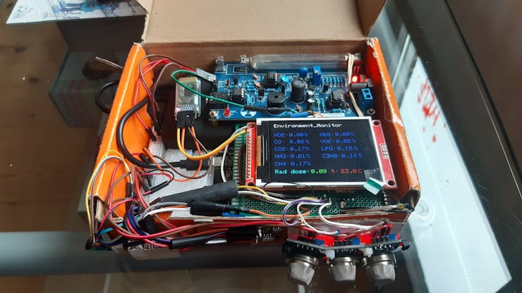
Arduino Mega 2560 is famous as most powerful board in Arduino line. It has 16Mhz core, 4 UARTs and significant number of analog and digital pins promising a wide range of possibilities. The sensor market for the average person is quite limited. In general, only gas sensors based on semiconductor properties are readily available for individual purchase. While their accuracy and usage range may not be as high as those used in professional settings, the price is generally quite affordable. Was decided to add TFT monitor with 2.8'' and 320x240 resolution to monitor measurements separately from a PC.
The common wiring diagram looks following:

As later became known, Arduino Mega is not much sufficient for project demands. It process all analog inputs too slowly, which was a significant drawback considering our expectations for higher speed. After reviewing the theory, we discovered that TFT sensors consume a significant amount of processing power, making the Arduino Mega 2560 board an less than ideal choice for this implementation. Since we didn't have access to STM32 or ESP boards, we decided to enhance our project through software improvements.Was modified the screen updating algorithm and implemented threading. The results were positive, and this approach worked quite well.
It worth to be mentioned about gas sensors. The MZH19B CO2 sensor is a member of the IR family of sensors, known for their accuracy. While not the most expensive option, it offers impressive precision. Equipped with UART and analog output, it also supports auto-calibration. Semiconductor sensors operate on the principle that the resistance of a semiconductor material varies depending on the concentration of the surrounding gas. These sensors participate in RedOx processes on the surface of the SnO2 semiconductor, leading to changes in its physical properties and, consequently, its electrical conductance. While manufacturers often claim a wide range of detection possibilities, many semiconductor gas sensors share a common active compound: SnO2. Although the surface film can be modified to allow for the detection of smaller molecules, these sensors generally lack intrinsic selectivity. As you can see, the signals from the MQ4 and MQ6 sensors are similar, exhibiting the same peaks and slopes, indicating that they react to pollutants in a consistent manner. Similar to the MQ sensors, Mics sensors are also based on semiconductor technology. However, I find them to be more qualitative in their measurements. As claimed by the manufacturer, selectivity is achieved through modifications to the semiconductor's surface. All Mics sensors have analog output, and their datasheets provide detailed information about the sensor's characteristics, including the measurement range, which is crucial for our research. It's important to note that all gas sensors require preheating and calibration under laboratory conditions. Since I didn't have access to these facilities, I established a zero point using clean air indexes and then calculated the differences between these values and those obtained at various locations.
In general, our device is capable of measuring various pollutants, including CO2, CO, CH4, LPG, C3H8, NO2, NH3, H2S, volatile organic compounds, and radiation levels using an Arduino Geiger counter kit.
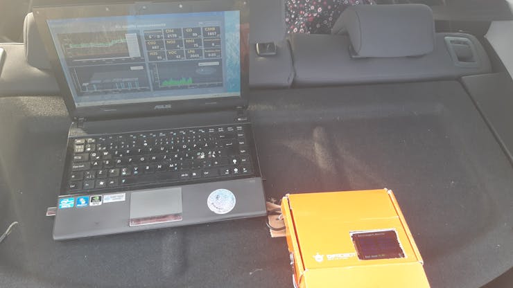
The device incorporates a Bluetooth HC-05 module, allowing for wireless data transmission to a laptop.

Qt software part
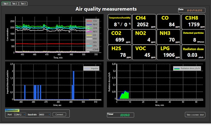
The main application designing was chosen to perform with C++ and Qt. On the one hand, maybe it would be better to combine Python and Qt, but was chosen other way.The extensive development possibilities, wide range of components, and strong community support have contributed to the widespread use of Qt. As a C++-based framework, Qt is seamlessly compatible with C++ code and can also be integrated with other programming languages.The C++-based application demonstrates high performance speed. Its primary requirements were the ability to capture data, visualize it in real-time plots, and save the data to a hard drive.
The result is following:

Test
To evaluate our device and accompanying software, we conducted several simple tests.
- A lit candle was placed in a sealed environment along with our device. As the candle burned, it released CO2, which we monitored.
- A lighter gas was sprayed onto the hydrocarbon sensors (CxHy).
The results of both tests are depicted in the plot below.:

As advertised by the manufacturer, the MH-Z19B CO2 sensor has a measurement range of 400-5000 ppm. During the CO2 test, the sensor readings rose to the 5000 ppm limit and then plateaued for over 60 seconds. However, the sensor eventually entered an error state and did not update its values until the board was reset.The behavior of the CxHy sensors is further illustrated in the same plot. The lighter gas is a mixture of propane and butane, with impurities of other hydrocarbons. As observed in the plot, the MQ4, MQ5, and MQ6 sensors exhibit similar responses to these compounds, suggesting that they lack selectivity.The rest of sensors did not respond to the CO2 or hydrocarbon spray.
MICs sensors from DFRobot exhibit similar characteristics to other semiconductor gas sensors but display some unique behaviors. For example, the MICS 5524 sensor can be used to detect a variety of gases, but it lacks specific selectivity for each gas. Instead, it generates a signal based on the general presence of gases in the air.
The rest of sensors were tested in natural environment.
Given that Denmark is widely recognized as one of the cleanest countries in the world, this research is particularly intriguing.
The measurement locations were selected as follows:
- Baltic Sea shore- Small town with moderate traffic- Countryside village- Kalundborg harbor- Kalundborg petroleum terminal- Kalundborg refinery plant- Baltic Sea shore in Ordrup village- Pig farm area
These diverse locations provide a comprehensive range of environments for assessing air quality.
As expected, the seaside area is generally cleaner, while traffic and farming areas are likely to have higher concentrations of CO2, CxHy, and other pollutants. I visited these locations and recorded measurements. The results were not as was expected.
Data set processing and results
As previously mentioned, our software collects data and stores it on the laptop's hard drive as JSON data sets in TXT files. These data sets (approximately 8000 data rows overall) can be processed using Python Pandas, allowing for the creation of plots for each location and subsequent comparisons.In few steps with manipulation with python pandas we have processed data and generated plots for pollutants and radiation level in current areas.
for item in record_data:
    data = []
    with open(item, 'r') as file:
        for line in file:
            timestamp, json_data = line.split(': ', 1)
            parsed_data = json.loads(json_data)
            parsed_data["timestamp"] = timestamp
            data.append(parsed_data)

    df = pd.DataFrame(data)
    df['timestamp'] = pd.to_datetime(df['timestamp'])
    dfs[item.split('.')[0]] = df

for filename, df in dfs.items():
    print(f"Data from {filename}:")
    print(df.head())
#
#
columns_to_iterate = ['C3H8', 'CH4', 'CO', 'CO2', 'H2S','LPG','NH3','NO2','VOC']
colors = ['b', 'g', 'r', 'c', 'm', 'y', 'k', '#FF5733', '#33FF57']
drap = df['DRAP']

for cols in columns_to_iterate:

    for i, (filename, df) in  enumerate(dfs.items()):

        last_ = df[cols].head(500)
        last_.plot(label=f'{filename}', legend=True, color = colors[i])
        avg_col = df[cols].mean()
        plt.axhline(y=avg_col, color=colors[i], linestyle='--', label=f'Average {cols}')

    plt.title(f'{cols} in different locations', fontdict={'fontsize': 16, 'fontweight': 'bold', 'fontfamily': 'serif'})
    #plt.legend(loc='upper right')
    plt.xlabel('Time, sec')
    plt.ylabel(f'{cols} Conc, ppm')
    plt.grid(True)


    plt.show()
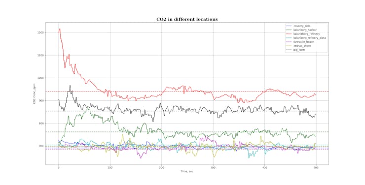
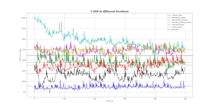
These following plots were retrieved:


Key Moments
1. A surprising finding was the Baltic Sea shore acting as a source of air pollution. Sea weed, which is laying on the sand whole year undergoes decomposition releasing H2S, methane and other hydrocarbon gases. It is visible on the plots above compering with other locations. To verify this observation, we conducted additional measurements in a different location, but the results remained consistent.
2. Surprisingly, the pig farm area appeared to be cleaner than the Kalundborg refinery plant in terms of the overall pollution index. While there was a slightly higher concentration of CO2 nearby, the plots did not indicate any significant presence of ammonium or other pollutants. Comparing farming and sea-weeds pollution the first one plays crucial role concluding from gigantic volumes of pig production.
3. Rural area considered to be clean. A presence of traffic is visible on the plots in increasing of hydrocarbons. A light increasing of CO2 might by caused by farming activity nearby.
4. As expected, the chemical plant leaves traces of its presence in the environment, as it's difficult to completely seal and isolate such a large-scale chemical production facility. Paying attention to the plot above, it is visible, that CO2 level is higher for 250 ppm then in rural area, it is approx 20%, that same about harbor area. Winds are spreading CO2 cloud to the town. About hydrocarbon gases, they are volatile, being lighter then air, presence of it less visible in Kalundborg town. However, overall, to state about exceeding concentration levels with MQ sensors data would be not right due to doubting quality and detection range, rightly would be to declare the concentration difference among several location. I guess, manufacturer stated detection range was inaccurate due to translation errors, and real gas concentration is 1000 times lower and relevant concentration is in ppb (particle per billion) units.


5. Granite is a key source of natural background radiation, containing uranium derivatives. Radiation levels may vary near building sites or granite processing plants. As shown in the plots below, a slight increase in radiation levels at the Kalundborg harbor (green plot line) could be attributed to the presence of granite in the area. However, overall, the radioactivity levels varied across different locations but did not exceed the natural background radiation limits.


Conclusion
For hobbyists interested in programming and device design, sensors from the QM and Mics series can be a good option from a price/quality perspective. However, they are not highly precise and have a limited range of concentration detection. For more accurate results with selectivity, there are numerous options available starting from $100 per item. About Arduino as hardware part, I presume, in this project it works on the edge of its possibilities. To update screen, read off 9 analog signals, process it and send data to the bt serial port - it is huge task and it has cope with it. But for tougher quests better to use stm32.
About Qt as framework and C++, really cool combination. I recommend it, if user wants to get application with max source efficiency, especially where sources are limited (embedded systems for instance).
To check out the source code you can on my GitHub page:
https://github.com/tech-science-club/Environment_monitoring
This article was first published on Hackster on October 21, 2024
cr: https://www.hackster.io/Dima_Panasenko/environment-monitoring-with-c-programming-dd3663
Author: Dima Panasenko


